Calibration Module

The pyccapt.calibration package provides workflows for atom probe tomography data preparation, calibration, reconstruction, and visualization.

Calibration visualization

Core Workflows

Typical calibration workflows include:

Import and crop datasets (HDF5, EPOS, POS, ATO, CSV, and raw-detector workflows).
Correct time-of-flight and estimate t0/flight-path parameters.
Convert time-of-flight to mass-to-charge (m/c).
Apply voltage and bowl corrections.
Perform 3D reconstruction.
Define and apply ranging windows, including saved .h5, .rrng, and .rng range files.
Generate 2D/3D visualizations and analysis plots.

Package Structure

core: validation, shared state, and primary calibration logic
data_tools: loading, conversion, and preprocessing utilities
mc: mass-to-charge and time-of-flight helper functions
reconstructions: reconstruction and structural analysis tools
clustering: clustering and isosurface workflows
leap_tools: LEAP/POS/EPOS/APT/RRNG/RNG readers, Cameca raw importers, and helper tools
tutorials: notebooks and notebook helper modules

Mass-Calibration Pipeline

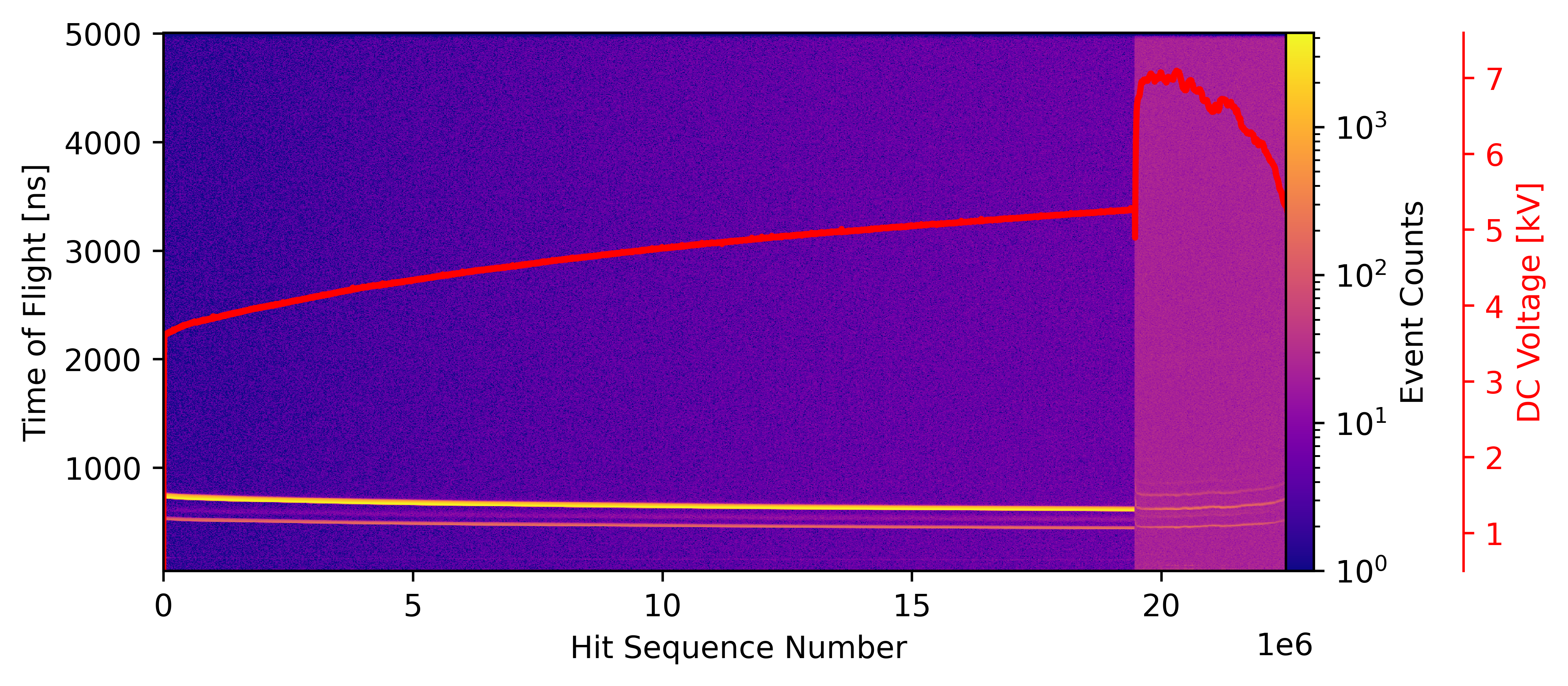
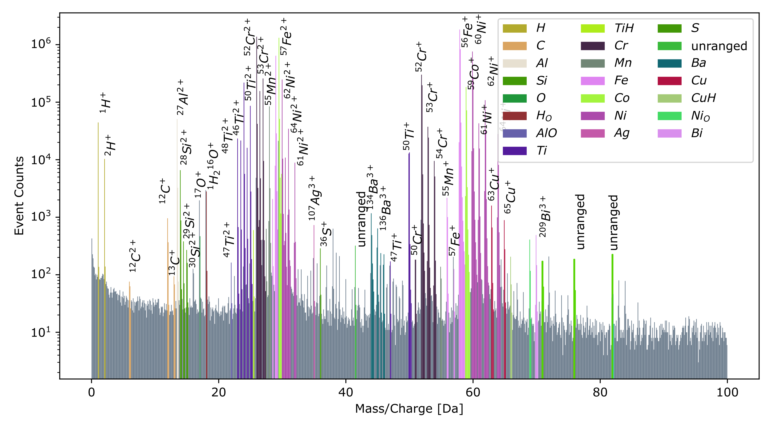
Mass calibration converts detector hits (time-of-flight, standing high voltage, detector position) into a calibrated mass-to-charge (m/c) spectrum. The pipeline in pyccapt.calibration.core.calibration runs the following stages in order:

Initial calibration — a global t0 and flight-path estimate converts time-of-flight to a first m/c.
Voltage correction — corrects each event’s m/c for the slow change in standing voltage during evaporation, fit over ion-index or voltage segments.
Bowl correction — corrects the residual position-dependent flight-time difference across the detector (the “bowl”), sampled in Cartesian or polar detector cells.
Time-drift correction (optional) — a multiplicative per-ion-index correction that cancels high-voltage or temperature drift remaining after steps 2-3 in long acquisitions.
Adaptive residual calibration — a per-peak temporal and spatial residual fit that tightens mass resolution after the parametric corrections.

Peak locations used to drive the fits are read at histogram bin centers, and histogram bins are anchored to the requested bin width.

Configuration presets

The data-processing notebook exposes a Config preset dropdown. All presets share the same voltage and bowl stages; they differ only in what runs afterward:

Adaptive residual (default) — voltage + bowl, then adaptive residual with the coarse-to-fine peak-scoring speedup.
+ time-drift correction (recommended) — adds the per-ion-index time-drift correction (stage 4) between bowl correction and the residual fit. Suited to long runs with measurable drift.
Legacy adaptive residual — voltage + bowl, then adaptive residual without the coarse-to-fine speedup. Slower, and reproduces the pre-2026 reference behaviour for bit-comparable results.

NIST reference fit

The ion-list helper provides a second Fit method that rescales the already-calibrated m/c onto reference (NIST) masses. It only rescales m/c; it does not re-fit the voltage, bowl, or drift corrections, so it composes with the pipeline above rather than replacing it. The rescale is applied to the current calibrated spectrum and is rejected automatically if it introduces non-finite values or collapses the mass spread.

Partial-Hit Recovery (Surface Concept)

A delay-line detector reports an event only when all delay-line ends fire within the hardware coincidence window. Pulses that fired some, but not all, channels are normally discarded. The Surface Concept raw-data workflow can recover physically valid hits from these partial pulses:

For each delay-line axis (x: channels 0+1, y: channels 2+3), candidate pairs are enumerated and a one-to-one assignment selects a consistent subset. Axes are cross-matched by time-of-flight agreement: a matched pair becomes a full 2-axis (xy) hit; unmatched pairs become single-axis (1-DLTS) partial hits.
The diagnostics path (extract_surface_concept_hits) enumerates every reconstructible pair and flags each one’s in_detector status against the configured detector limit, so out-of-detector reconstructions are reported rather than silently dropped.
The live merge path (data_tools.partial_recovery.merge_partial_tdc_into_dld) appends the recovered rows to the /dld dataframe, tagging each with a dlts (2 or 4) and dlts_quality label. Single-axis recovered rows carry NaN on the unrecovered detector axis. Pulses are grouped by event_group_id (wrap-safe), not by the raw start_counter, which wraps during long runs.
3-of-4 (time-sum) recovery (on by default in the merge path): pulses that fired one complete delay-line axis plus a single end of the other axis are promoted to full (x, y) hits. The crossed delay lines share the same total propagation time (t0 + t1 = t2 + t3), so the missing end is sum_complete_axis - t_present; the recovered hit is gated by non-negative recovered times, the detector radius, and the ToF window, and labelled dlts_quality = recovered_xy_3of4. The Surface Concept firmware “quadrupel finder” requires all four stops, so these hits exist only after this offline step. Set recover_three_channel=False to disable it.
Matched multi-hit residual recovery (opt-in, recover_from_matched_multihit=True): the firmware keeps one hit per pulse, so a matched pulse that fired more stops than its DLD event(s) used may hold a second ion. The stops the firmware used are inverse-matched to its DLD event(s) by a coherent quadruplet – a (ch0, ch1) pair within multihit_match_tol_cm of det_x and a (ch2, ch3) pair within multihit_match_tol_cm of det_y whose ToFs agree and whose combined ToF matches the firmware event’s recorded t (ns) – and removed; the residual stops are run through the recovery above. The ToF match matters because a detector coordinate depends only on the per-axis time difference, so a second ion at a similar position but a different flight time would otherwise be mis-removed; keying on the recorded flight time prevents that. It is opt-in because the inverse match is heuristic – a pulse with no coherent quadruplet matching the firmware event is skipped, avoiding both double-counting the firmware’s own hit and stitching a cross-ion artefact (a firmware hit that was itself a 3-channel reconstruction therefore skips safely).
Order preservation: recovered atoms are inserted into the DLD frame at their acquisition position (right after the native rows of the most recent preceding pulse), never by sorting on start_counter (a periodic counter whose value repeats throughout a run), so the reconstructed z/depth sequence is preserved.
Only full (x, y) hits are merged by default; single-axis 2-DLTS partials (one detector coordinate is NaN) are excluded because they cannot be placed in the 3-D reconstruction. Set include_one_d_partials=True to also append them (they appear in the mass spectrum via a centred-axis mc estimate).

Partial-hit recovery is available from the raw_data_analysis.ipynb notebook and through the auto raw-analysis helper.

For a step-by-step walkthrough — the delay-line reconstruction formulas, worked examples of Surface Concept pulses of every length (0–8+ stops), the matched multi-hit residual recovery, and the TDC↔DLD match-quality cross-check printed at load time — see RAW_DATA_ANALYSIS.md.

Shared State and Validation

Calibration workflows use shared mutable state through Variables in pyccapt.calibration.core.share_variables. Validation and state-related errors should raise explicit calibration exceptions.

Cross-Platform Paths

Use pyccapt.calibration.path_utils helpers for output and figure paths:

ensure_directory
build_output_path
save_figure

Data Structures

Calibration and range-file schema details are documented in Calibration_DATA_STRUCTURE.md.

Tutorials

Interactive examples are available in:

pyccapt/calibration/tutorials/jupyter_files
pyccapt/calibration/tutorials/colab

The main Jupyter widget workflows currently include:

data_processing.ipynb
visualization.ipynb
L_and_t0_determination.ipynb
raw_data_analysis.ipynb
cameca_raw_import.ipynb
reflectron_correction.ipynb
tapsim_node_builder.ipynb

A batch CLI companion to the reflectron notebook is also available: python -m pyccapt.calibration.reflectron_correction.batch_cli scans a folder for .epos files and writes <stem>_corrected.h5 (and optionally .epos) beside each input for a chosen instrument preset. See the Reflectron Batch Correction (CLI) tutorial page for arguments and examples.

Speeding up calibration with multiple workers

A handful of calibration hot paths (bowl correction polar sampling, voltage correction segment loop, Surface Concept raw-data diagnostics) automatically parallelize across CPU cores when the workload is large enough to amortize executor startup. The default is auto; set PYCCAPT_PARALLEL_WORKERS=1 to force serial (useful for reproducible benchmarks and CI). See the Parallel Execution in Calibration tutorial page for the env vars, measured speedups, and which paths benefit.

Running on small-RAM machines

The calibration pipeline ships a memory-mapped I/O layer (pyccapt.calibration.data_tools.lazy_io) so multi-gigabyte EPOS / POS / pyccapt-raw HDF5 files can be loaded, reflectron-corrected, and analyzed on machines with as little as 8 GB of RAM. The reflectron batch CLI uses it automatically (peak heap drops from multiple GB to ~270 MB), and the raw-data widget exposes a Low memory checkbox that routes the stats through chunked code paths. See the Working with Big Datasets on Small RAM tutorial page for the full design, opt-in entry points, and measured before/after numbers.

Google Colab support is currently provided for:

data_processing.ipynb
visualization.ipynb

The tutorial save steps can export processed datasets as HDF5, EPOS, POS, and ATO. The visualization helpers also include Min-Max and Maximum-Separation clustering, iso-surface generation, and proxigram analysis for selected precipitate populations.

Linking and saving raw `/tdc` data alongside `/dld`

PyCCAPT acquisition files contain both a /dld group with reconstructed events and a /tdc group with the raw delay-line timestamps (DLTS) from which those events were derived. From the calibration tutorials you can opt in to loading both groups together via the Load raw tdc dropdown, and at save time choose Save raw tdc to write the still-relevant raw rows into a /tdc key inside the calibrated .h5 output.

Internally this is handled by a shared event_group_id column added to both dataframes when the file is loaded with load_tdc_raw=True. The column rides through every cropping step in the calibration workflow (TOF clip, ROI, FDM, sequence range, manual mask drops); at save time the linked tdc rows for deleted dld rows are dropped, while orphan tdc rows (pulses that never produced a reconstructible dld event) are always preserved. See Calibration_DATA_STRUCTURE.md for the on-disk schema of the optional /tdc group and the linking semantics.

The user-facing tutorial pages are grouped in the Tutorials section of this documentation set.